Greg's supplementary notes
Visual Variables
The followin table is a simplified summary of "visual variables" paper, with some modifications.
| variable | grouping | quantitative |
|---|---|---|
| position | 3 | 3 |
| size | 3 | 2 |
| shape | 1 | 0 |
| H/S/B | ? | 1 |
| orientation | ? | 1 |
| texture | ? | ? |
- "associative" => "grouping"
- "quantitative" + "order" => "quantitative" implies "order" but not vice versa
- "length" => "resolution"
- "color" + "value" => "HSB", i.e. hue + saturation + brightness
Building and running rawgraphs docker
You could use the cloud version
of rawgraphs directly if your data is not sensitive.
Here we will build our own local version for complete privacy.
Visit here.
Then in terminal, sudo bash and do the following:
docker ps -a
mkdir ~/rawgraphs-docker
cd ~/rawgraphs-docker
wget ...
docker build -t rawgraphs .
# take quite a while
docker run -d --name rg0 -p 3072:3000 rawgraphs
Then use the browser to visit localhost:3072 . It may take quite a while for the docker to show the first web page.
Preparing "electricity mix" dataset from BP and EMBER (2022)
A. 3-letter country code
- Data: owid ; Greg
- Greg's version was generated by processing owid's version using country-encode.py. See blog post (zh_TW)
-
( head -n 1 electricity-mix.csv ; grep -P '^\w+,Asia,' electricity-mix.csv ) > em-asia.csv
( head -n 1 electricity-mix.csv ; grep -P '^(CHN|DNK|DEU|IND|IDN|JPN|KGZ|MNG|SWE|TWN|USA|VNM),' electricity-mix.csv ) > em-some-countries.csv
( head -n 1 electricity-mix.csv ; grep -P ',2020,' electricity-mix.csv ) > em20.csv
B. Hierarchy of electricity sources
( head -n 1 electricity-mix.csv ; grep -P '^USA,' ) > em-usa.csv- Open em-usa.csv using libreoffice, make all fields narrower, freeze first row, "wrap text" on 1st row, delete every column starting from "carbon intensity ...", save as .ods .
-
Make hypotheses about categories of electricity energy sources, and use arithmetics to verify them. => usa-check.ods
- From the full csv file (containing all countries) delete unwanted columns, rearrange the remaining columns, and simplify the header to create: electricity-mix-leaves.csv
- Upload electricity-mix-leaves.csv to rawgraphs. Try "multi-set bar chart" and "stacked bar chart".
- Run melt.py to produce electricity-mix-melted.csv
( head -n 1 electricity-mix-melted.csv ; grep ',2021,' electricity-mix-melted.csv | grep -v ',imports,' ) > emh.csvperl -pe 's/,(coal|oil|gas),/,fossil,$1,/; s/,nuclear,/,nuclear,nuclear,/; s/,(hydro|solar|wind|bio|other),/,renewable,$1,/' emh.csv > emh2.csv- Edit emh2.csv and add a header "category" for the new column created above.
- Upload emh2.csv to rawgraphs. Try "treemap", "sunburst", "circle packing", and "circular dendrogram".
Q: What if we are to plot the "per capital" columns? Does treemap make sense?
Preparing a few data sets as csv or as sqlite3 db
A.
- Finding bloatware on android (zh_TW) => csv, plot
- List of natural satellites => csv,
plot
wget https://en.wikipedia.org/wiki/List_of_natural_satellites -O natural_satellites.html
python3 html2csv.py natural_satellites.html > natural_satellites.csv
# manually remove redundant info in natural_satellites.csv
perl -pe 's/±[\d\.]+//g ; s/\[\d+\]//g ; s/\s*\(r\)//' natural_satellites.csv > a.csv
perl -pe 's/"(\d+),/"$1/g ; s/"(\d+),/"$1/g ; s/"//g' a.csv
- sql join review; Import CSV into SQLite, with numerical columns: export as CSV; example: sales.csv from chinook.db
B. Electricity mix per capita
wget https://ckhung.github.io/a/m/23/em/electricity-mix-pc.csv- In sqlite3:
.mode csv
.import electricity-mix-pc.csv main
.schema
- Copy the output of .schema (the "CREATE TABLE" statement) to some text file, edit to change the type of "Year" to INTEGER, and the type of every column afterwards to REAL.
- Back in the sqlite3 session:
drop table main;
-- now paste the modified "CREATE TABLE" statement
.import electricity-mix-pc.csv main
.save em-pc.db
metabase
- Downloading and running jar file
- getting started with metabase
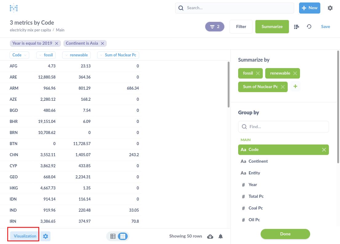
- Import the em-pc.db sqlite database. (See below, two pictures on the left.)
- Create a new "question"
- Pick the em-pc.db database, the main table.
- Add filters: year equal to 2019, continent is "Asia"
- Add summery metrics: custom expression: sum of Nuclear Pc, "sum([Coal Pc] ) + sum([Oil Pc] ) + sum([Gas Pc] )" named "fossil", and "sum([Solar Pc] ) + sum([Hydro Pc] ) + sum([Wind Pc] ) + sum([Bioenergy Pc] ) + sum([Other Pc] )" named "renewable".
- Group by "code".
- Click "visualization" at lower left corner, select "scatter", click the "gear" icon at the bottom next to "visualization".
- Set bubble size to "Sum of Nuclear PC", X-axis to "renewable", and Y-axis to "fossil".
- Save the question and give it a name.


grafana
- github
- install, then go to localhost:3000
- forgot password?
- config file location: /etc/grafana/grafana.ini
- Install csv datasource and modify /etc/grafana/grafana.ini, then
systemctl restart grafana-server(local path?) A csv data file must not contain extra spaces! - Start from "Configuration" => Data Sources. Then go to "Explore" to define some fields so that they never get ignored.
- From "Dashboards" => "Browse" one can manage all dashboards. A dashboard may contain several panels.
- From a panel's context menu one can choose "Edit". On the upper-right corner, one can choose the type of chart to display. There are a lot of chart types (e.g. bar chart, histogram, ...), but unfortunately bubble chart is not one of them. Then on the right hand side there will be lots of configuration options for that specific type of chart.
- more tutorials
linechart using gnuplot
(head -n 1 electricity-mix-leaves.csv ; grep '^GBR,' electricity-mix-leaves.csv) > em-uk.csv- In gnuplot,
load "em-uk.gpt" - Also try:
load "em-uk-stacked.gpt"But stacked line chart may not be a good chart for conveying information visually.
Bubble chart using gnuplot
Copy and rename these three datasets from OWID: "Global Data Set on Education Quality (1965-2015) - Altinok, Angrist, and Patrinos (2018)", "Press Freedom - Reporters sans Frontieres (2019)", "World Happiness Report (2021)".
python3 keep-latest.py education.csv > edu2.csv
python3 country-encode.py edu2.csv > edu3.csv
grep ',Asia,' edu3.csv | cut -d, -f 1,3,5- | sort > edu4.csv
# similar processes for the other two data sets
join -t, -a 1 -a 2 prfr4.csv happy4.csv | join -t, -a 1 -a 2 - edu4.csv > combined.csv
Use libreoffice to open combined.csv , manually add the header row back, and delete unnecessary columns. Finally in gnuplot:
set datafile separator ","
set xlabel "press freedom"
set ylabel "edu: avg"
plot "combined.csv" using 3:5:($4*1) with points lt 1 pt 6 ps variable title "happiness", "combined.csv" using 3:5:1 with labels title ""
Try to use different columns as X and Y axes.
jq
- Your json data go through a series of functions or operators connected by pipes "|".
- At each stage the data is either a number, a string, an array, an object, or a stream of several strings/arrays/objects (see below)
- At each stage you can use "." to refer to the current data. (Think of "self" in OOP.)
- Some functions take "." as the implicit argument
and therefore you don't even need to mention "."
when calling such functions.
For example:
echo '[2, 3, 5]' | jq 'add / length'computes the average of an array. - The
map()function transforms every element of an array into something else. Think of its "argument" as the return value -- it's actually the output, not the input. For example,echo '[1,2,3]' | jq 'map(.*.)' - Empty [] appended to an array or an object is called the "Array/Object Value Iterator". It returns all elements of an array, or all values of an object. The return value is called a stream. Do not think of a stream as an array. Let's say the next function or operator downstream the pipe is f. jq does not apply f to the stream as a whole. It iterate over the stream and apply f to each value of the stream,
- The "as" syntax only adds a variable definition to jq's memory. It passes the input along unchanged as output to the downstream function.
- The input data to
@csvmust be a stream of arrays. each of which is treated as a row. For example:echo '[[1,2,3], [2,4,6], [3,6,9], [4,8,12]]' | jq -r '.[] | @csv'Another example:jq -r 'map([.StopName["Zh_tw","En"]])[] | @csv' 151-stops.json - Now you can understand how to convert json to csv using jq.
- It may be easier to break your job into separate steps. Write a simple jq command to process your data and redirect the result into a file. Then process that file with the second jq command.
Ubike rental points: from TDX to umap
A. umap
- Sign up an openstreetmap account.
- Sign in to umap using your OSM account. At the bottom there is a menu to change the language.
- Look at some of ckhung's maps and get familiar with umap.
- The "share" button On the left hand side can be used to download map data as geojson file.
B. downloading from tdx
- The ministry of transportation releases a lot of data at the TDX website. We are interested in bike rental stations
- Choose a city, let's say "台中市". Clear "$top" (we want all, not just top 30). Make sure "$format" is json. Click "Execute". Click "Download". Let's say we save the file as "tc-ubike.json" . Take a look at tc-ubike.json .
C. converting to geojson
jq 'map(.StationName.En)' tc-ubike.jsonjq 'map( { type: "Feature", geometry: { type:"Point" }, properties: { name:.StationName.En } } )' tc-ubike.jsonjq 'map( { type: "Feature", geometry: { type:"Point", coordinates:[ .StationPosition.PositionLon, .StationPosition.PositionLat ] }, properties: { name:.StationName.Zh_tw, description:.StationName.En } } )' tc-ubike.json > tc-ubike.geojson
D. uploading to umap
 In umap, create a new map.
- Click the pen icon in the upper right corner to start editing the map.
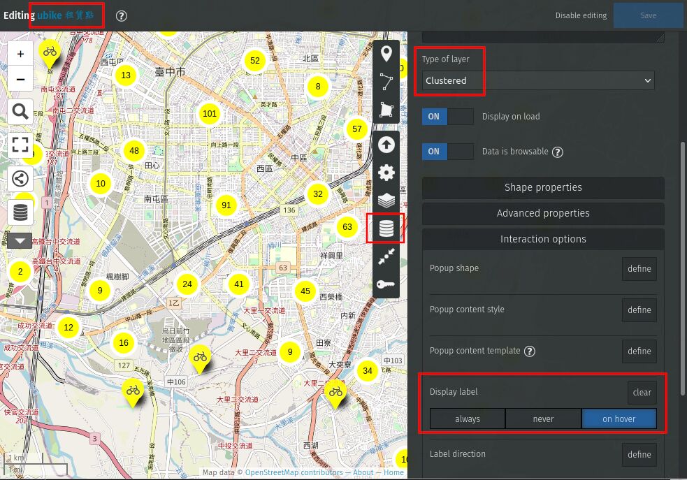
- (optional: You can click the upper left corner to change the map name.)
- On the right hand side, click "import data", browse to choose tc-ubike.geojson, Then "import".
- On the right hand side, click "manage layer". Click the pen icon for the newly created layer "tc-ubike.geojson" to edit this layer.
- Change "type of layer" to "clustered".
- "interaction options" => "display label" => "on hover"
Bus data preparation
Download ptx-example.bash . Also see explanation in zh_TW.
source ptx-example.bash 'https://ptx.transportdata.tw/MOTC/v2/Bus/DisplayStopOfRoute/City/Taichung/151?%24format=JSON' > 151.json
jq -r '.[2].Stops | (.[0].StopName | keys_unsorted) as $keys | $keys, map([.StopName.Zh_tw, .StopName.En])[] | @csv' 151.json > 151-stops.json

jq '.[] | select(.RouteName.En=="151")' taichung-bus-sched.json
jq '.[] | select(.RouteName.En=="151" and .Direction==1)' taichung-bus-sched.json
jq '.[] | select(.Timetables[0].StopTimes[0].StopName.En=="Chaoyang University of Technology")' taichung-bus-sched.json
jq 'map( select(.Timetables[0].StopTimes[0].StopName.En=="Chaoyang University of Technology") )' taichung-bus-sched.json
jq 'map( {"RouteName":.RouteName.En, "Timetables":(.Timetables|length)} | select(.Timetables>40) )' taichung-bus-sched.json
jq 'map( {"RouteName":.RouteName.En, "Frequencys":.Frequencys} | select( .Frequencys != null ) | .RouteName )' taichung-bus-sched.json
When the jq syntax becomes too complicated,
you can consider writing a small python program,
for example, to list all routes that either has "Frequencys" info or
has more than some number of trips listed in "Timetables":
python3 freq.py -n 40 taichung-bus-sched.json
Converting json to csv using zq
ZED is a versatile structured data processer. It can process json and csv files and has its own zson format, among other things. We will try to convert tcbus/151.json to a csv file containing only interesting fields to illustrate how to use zq. See tutorial and language definition for more information.
In one terminal tab or window:
zq -f json 'this[1].Stops' 151.json | jq . | less
to see the input data. In another terminal tab or window
try the following:
zq -f csv 'this[1].Stops | over this => (yield StopName)' 151.json
zq -f csv 'this[1].Stops | over this => (yield {StopName, StopPosition})' 151.json
zq -f csv 'this[1].Stops | over this => (yield {name:StopName.En, lat:StopPosition.PositionLat, lon:StopPosition.PositionLon})' 151.json
You may want to add " | jq . | less" at the end of each command for easier reading.
When your input data file is huge, be sure to specify
the input file format (-i json) to make zq's work easier.
Then you can add a comparison expression to
filter/pick only the element you want:
wget https://v.im.cyut.edu.tw/ftp/22/taichung-bus-sched.json.gz
gunzip taichung-bus-sched.json.gz
zq -i json -f json 'over this | RouteName.En=="151"' taichung-bus-sched.json
zq -i json -f json 'over this | RouteName.En=="151" and Direction==1' taichung-bus-sched.json
zq -i json -f json 'over this | Timetables[0].StopTimes[0].StopName.En=="Chaoyang University of Technology"' taichung-bus-sched.json
![[rss feed 圖案]](/~ckhung/i/rss.png)